The Power of Conditional Simulation in Mineral Resource Evaluation

Discover the Power of Conditional Simulation in Mineral Resource Evaluation and why it is crucial for risk assessment and informed decision-making. Our article explores simulation methods and highlights its value in mineral resource estimation and evaluation.

Introduction

The Power of Conditional Simulation in Mineral Resource Evaluation is crucial, playing a significant role in assessing associated risks. In this context, probability serves as a measure of risk, such as in the case of determining the likelihood that a given ore block is above an economic grade cut-off. By creating multiple, equally probable realisations of spatially distributed data based on known data points, conditional simulation enables mining teams to make informed decisions about mining and processing methods.

The primary purpose of conditional simulation is to capture the uncertainty associated with spatial prediction and to provide a range of possible outcomes or scenarios, instead of a single prediction. The uncertainty inherent within sample data often leads to many potential interpretations, while conditional simulation provides the opportunity to understand and quantify this uncertainty, allowing quantifiable risk-based decision making. In particular, conditional simulation can help you determine which parts of your deposit should be mined as a matter of priority or highlight areas where you may need more data for confident decision making.

In this article, we discuss the intricacies of geostatistical conditional simulation and explore its applications in mineral resource evaluation.

Understanding the Conditional Simulation in Mineral Resource Evaluation

A Comprehensive Explanation of Conditional Simulation

Conditional simulation is used in various fields, including hydrogeology, environmental studies, oil and gas studies, mining, and geology. In mining, it is most commonly used to assess grade variability in an ore body, whereas in hydrogeology, it may be used to estimate the distribution of groundwater levels or the concentration of contaminants in groundwater. The oil and gas industry can use conditional simulations of static models to analyse the performance of different reservoir simulation scenarios.

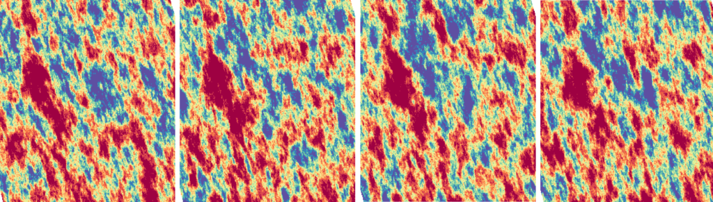
The primary objective of conditional simulation in resource estimation is to generate multiple equi-probable realisations (i.e. multiple models with equal likelihood) of a property, such as mineral grades or ore quantities, that are consistent with available data and honour the distribution and spatially correlated patterns observed in the geology. These realisations represent equally probable scenarios that reproduce all features of variability and spatial continuity within the data.

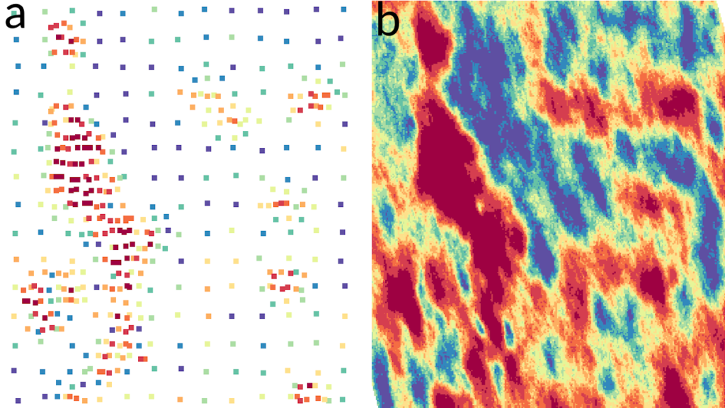
The process of conditional simulation begins with a standard analysis of the available data, which includes domaining and modelling the characteristics of the deposit. Declustering may also be necessary for clustered data for proper validation during the post-processing steps, as well as for transforming the input data into Gaussian equivalent values or normal scores. Data transformation is particularly important because most commonly used geostatistical techniques for conditional simulation assume the data has a Gaussian distribution. As such, the variogram model must be fitted to the Gaussian transformed data for use in the conditional simulation. During simulation, a grid of points, referred to as nodes, are informed (host the simulated values) to create the point simulated data. Where available, the existing geological block model should be used to correctly distribute nodes within the known domain volumes.

During simulation, the overall method and kriging type are important decisions which can have a direct impact on the quality of the simulations, depending on the underlying relationships in the data. Correct selection of methods, along with other estimation parameters, such as the search neighbourhood, ensures that the simulation results properly reproduce the input data characteristics.

Point data is converted to block volumes, or “block models”, through a process called reblocking. Each block contains at least one simulated data point, with the simulated block grade given as an average of the simulated values within the block. Defining a grid size of sufficient density so that there are a suitable number of nodes inside the block is important, as these nodes represent an appropriate discretisation of the block. However, the larger the number of nodes, the longer the simulation will take to run.

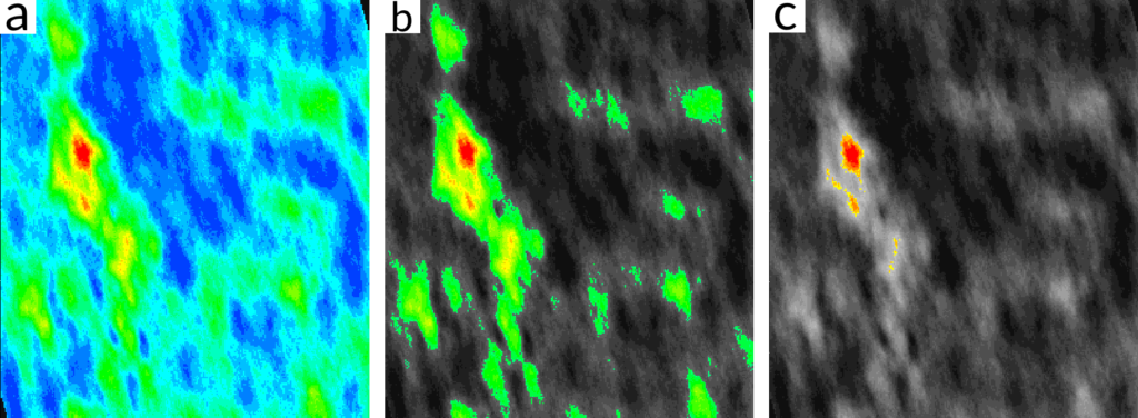
The simulation results can be assessed using post-processing tools, such as grade tonnage curves for the volume and grade of material that may be obtained at different cut-off grades, and probability plots that illustrate the probabilities of individual blocks at defined grade thresholds. Particular attention should be given to areas where there is very little variability, compared to areas of very high variability, which may represent areas that could benefit from additional sampling. Finally, the interpretation of the simulations should be kept in context of your appetite for risk. For example, a 60% likelihood of ore for a block may be appropriate for one operation, but not for another.

Comparing Methods of Conditional Simulation

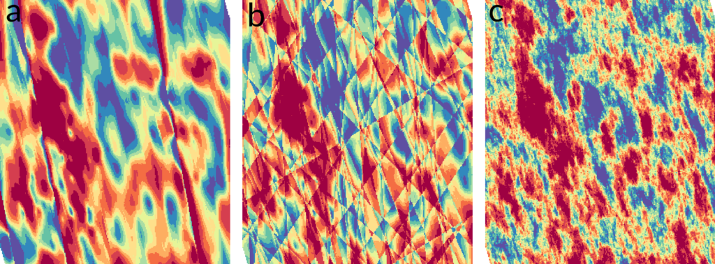
There are several conditional simulation techniques proposed in the geostatistical literature. In this post, we will have a look at the three most common methods for conditional simulation used in the Mining industry: Sequential Gaussian Simulation, Sequential Indicator Simulation and Turning Bands.

• Sequential Gaussian Simulation (SGS) – SGS is primarily used to simulate grades. This method requires the input data to be transformed into equivalent Gaussian values and assumes the data has a Gaussian distribution with a fixed mean of 0 and a variance of 1. The Gaussianity assumption allows us to determine the distribution of the grade at an unsampled location based on the observed values at nearby locations. This distribution is Gaussian with the mean and variance values equal to the simple kriging estimate and corresponding kriging variance, respectively. Simulated grades are then calculated sequentially by selecting one location at a time and simulating its value using the observed values at nearby locations. The sequential process means that previously simulated nodes are used to obtain the kriging estimate and its variance, if they are part of the nearby locations of the unsampled location being simulated. Gaussian simulated results are back-transformed to input data space for validation, which can then be used for further analysis.
  
• Sequential Indicator Simulation (SIS) – SIS is primarily used for simulating categorical values, unlike SGS, which generates values for continuous data. In principle, SIS is similar to SGS, except that the simulated data is transformed to a binary distribution rather than gaussian, either by coding the categories to membership (e.g.1 if a member of the category, 0 if not), or by defining a threshold for continuous data to be coded (e.g.0 below the threshold, 1 above). The simulation process is otherwise much the same, and multiple categories, or thresholds can be run individually and then recombined with post-processing to create the final simulation result.
  
• Conditioning by kriging with Turning Bands simulation – Like SGS, this method requires the input data to be transformed into equivalent Gaussian values and assumes a multivariate Gaussian distribution. However, contrary to SGS, turning bands uses a two-step approach. Firstly, a non-conditional simulation is generated using the turning bands simulation approach. Secondly, the conditioning takes place by combining the simple kriging estimate of the data and the simple kriging estimate of the difference between the data and the non-conditional simulation. This process guarantees a conditional simulation is obtained. Turning Bands generates random realisations of spatial data by dividing the simulation process into bands or sections. In the past, these bands could create unwanted artifacts in the final models. However, modern computing techniques have largely overcome this issue through an increased capability to run more bands, thus reducing the impact of each individual band on the final model.

Advantages of using Conditional Simulation in Geostatistics

The key benefit of using conditional simulation in resource estimation is that it allows you to determine the risk involved in estimating your resource grade and volume, by understanding the uncertainty throughout your deposit. Some other advantages are:

• Variability Quantification at Multiple Scales – Conditional simulation allows you to quantify the spatial variability of a deposit, which standard techniques, such as kriging on its own, often fail to provide. It also accounts for the variability seen at smaller scales, even when the available data is large-scale.
• Decision-Making and Financial Risk Assessment – Quantifying the risk associated with the deposit assists in making strategic decisions, like mining sequence, financial and feasibility scenario analyses, and drill spacing. Geological uncertainty can also be linked to economic outcomes to better evaluate the financial risks associated with mining projects.

Disadvantages & Possible Pitfalls of Conditional Simulation

Conditional simulation is an invaluable tool for mineral resource estimation, but, like any geostatistical method, it’s important to remember that there are some potential drawbacks. It’s also important to note that the realisations and outputs given as part of conditional simulation need to be thoroughly validated to ensure that they make sense for the deposit. Some potential drawbacks and considerations include:

• Uncertainty – While conditional simulations can provide estimates of uncertainty or risk, it’s important to remember that these are based on the spatial models (variograms) and data. If the model or data are of poor quality, the uncertainty estimates may not be reliable.
• Assumptions – The world rarely follows all theoretical rules, especially when it comes to estimation. If the assumptions of the conditional simulation techniques don’t hold true, the results of the simulations may be compromised. Validation of the results is extremely important for early identification of any issues that may arise during the simulation process.
• Workload and processing time – Processing, validating and using conditional simulations requires more time and effort than running an estimate. Furthermore, large conditional simulations consume the computer resources and disk space. While the results of conditional simulation can be extremely beneficial, this must always be weighed up against the pressures of delivering the right information at the right time.

Despite these potential drawbacks, conditional simulation remains an extremely useful method in geostatistics. It offers the ability to generate multiple, equally probable realisations that honour the data and its spatial relationships, providing a measure of the uncertainty and risk associated with a resource estimation.

Conclusion

Conditional simulation is a vital tool that brings a wealth of insights to any mineral resource estimation. It allows the quantification and visualisation of the spatial uncertainty in a deposit. By generating multiple equally probable realisations and summarising the results, resource geologists can make more informed decisions regarding resource extraction strategies, investment decisions, and risk management. However, conditional simulation’s reliability relies on data quality, spatial models, and the ability of the user to determine the most appropriate methods for their deposit. Despite these challenges, conditional simulation empowers professionals to navigate the complex terrain of grade and geological uncertainty.

For streamlined and user-friendly conditional simulation workflows, see more about Supervisor’s accessible geostatistics by clicking the below button.

If you’re interested in learning more about conditional simulation, Snowden Optiro offers several short courses on this topic, as well as many others in the areas of geology and geostatistics. Click the button below for more details.